Turning the jungle into punch cards
During the early optimistic days of the summer 2020 quarantine I watched Ken Burn’s fantastic 10 part 18-hour series on the Vietnam war. It is by far the most accessible and compressive body of work on the subject. Burn’s starts you off pre-WWI so you really get a comprehensive picture of things.
One of the aspects of the war that fascinated me the most was the push by the the then Secretary of Defense, Robert McNamara, to quantify as much of the war as was computationally possible. One of the most storage intensive of McNamara’s efforts was the Hamlet Evaluation System, which attempted to quantify the degree to which ~12,000 small, rural Vietnamese villages had been pacified. A RAND corporation report found the program was producing 90,000 pages of data every month. More than could have ever been useful.
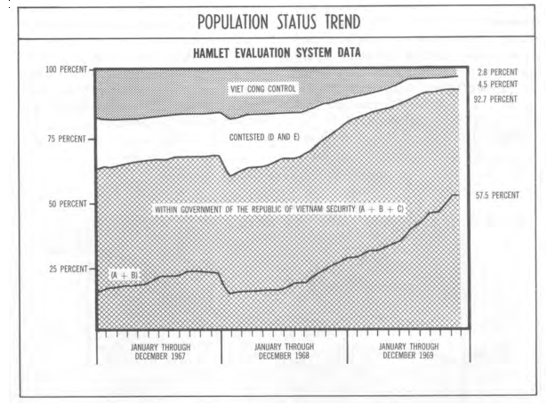
Example of data produced by the Hamlet Evaluation Program showing change in hamlet classifications over time
This was the data produced by just one wartime metrics program. Even if the DoD had the raw 60s era computing power and the army of FORTRAN programers that would have been needed to wrangle it all, the metrics themselves were questionable at best. One of the historians interviewed as apart of Burn’s series said something along the lines of “When you can’t measure whats counts, you make what can count the measure”.
I was interested in actually seeing what that data looked like in its raw form. What where programmers of the era actually looking at and wrangling when some Army big-wig said “We need to be producing 90,000 pages of data a month”? So I did some googling and dug into a couple documents hosted my the National Archives to try and get a picture of what Vietnam looked like from the perspective of a punch card.
The Phung Hoang Mangement Information System
The degree of documentation relating to the Hamlet Evaluation System that survives to today is, somewhat unsurprisingly, extremely large. So picking one out to dive into was a less than analytical process.
A came across the Phung Hoang Mangement Information System, PHMIS, (MACV Document Number DAR R33 CM-01A, March 1972) which was later replaced with the National Police Infrastructure Analysis Subsystem; a database cataloging the personal information of Vietnamese who where suspected of or convicted of aiding communist forces as part of the Hamlet Evaluation Program. This entry was interesting to me because it had both the technical documentation needed to actually make sense of the data and because of its historical context. The PHMIS was used as a catalogue for the operations of the Phoenix program a CIA headed counter-insurgency operation that among other techniques, employed torture and assassination to identify and kill Viet-Cong and Viet-Cong collaborators.
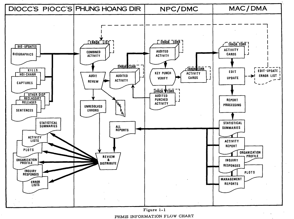
Flowchart depicting data schema of the Phung Hoang Mangement Information System, March 1972 report
The Phoenix Program was, deservingly, a locus of controversy within a storm of controversies surrounding US operations in Vietnam, eventually building to a series of congressional hearings in 1971. The data stored in this National Archive entry, in some way, is the bureaucratic reflection of all the individual stories and lives impacted by this corner of red-scare induced mania.
Getting into the data
The PHMIS National Archive entry contains one main data file and some aggregated technical documentation.
RG330.PHMIS.P6972: The actual binary data file. Refered to asRG330222.1SPA.pdf: Historical background on the PHMIS222.1DP.pdf: Technical documentation on format ofRG330
At first I was a bit lost as to where to start after thumbing through the technical
documentation. At first I naively tried to read RG330 as UTF-8 but then
soon remembered unicode was not created until the 1980s.
Thankfully I found the technical specifications summary provided by the National Archives which had this critical information.

The number of records, the length of each record and critically the encoding: EBCDIC. At this point I had no idea what EBCDIC encoding was but some quick googling corrected that. Basically, EBCDIC (Extended Binary Coded Decimal Interchange Code) was created by IBM in the late 1950s and used a perplexing (see EBCDIC wikipedia page criticism and humor) eight-bit character encoding for mainframe computers.

Example of EBCDIC encoded punch card.
I almost stopped here, but the Python community came through once again and thanks to Thomas Aglassinger you can successfully run the command
pip install ebcdic
and have a number of EBCDIC encodings to work with right in Python. And the
secrets of RG330 can be revealed in their UTF-8 glory with the Python
snippet below.
import ebcdic
filepath = './RG330.PHMIS.P6972'
data = open(filepath, 'rb').read().decode('cp1141')
Wrangling
The next step was to get the decoded mass of information into something
that could be output to a csv file and would be much easier to work with. The
technical documentation that let us know RG330 was EDCDIC encoded also says
that the record length is 319 so my approach was to go with that and pray to
the data-wrangling Gods.
step = 319
print(data[:step])
gives
01000005A207000069120H691270122E70125041100002CB 34KKKKK5C12070103001BM########################00000ä 00000ä 00000ä 00000ä 00000ä 00000ä 00000ä 00000ä 0ä ########################################################################
which as a first attempt does not actually look that bad. The National Archives
documentation notes that a personally identifying information in the database
has been redacted for public use - which is showing up as the # characters.
A memo from December 10, 1992 states the following.

I used this to verify the correctness of my naive parsing approach. If everything lines
up, the only characters we should be finding in columns 73-96, 248-271, 272-295
and 296-319 are #s.
redacted_base_1 = [(73, 96), (248, 271), (272, 295), (296, 319)]
redacted_base_0 = [(r[0] - 1, r[1]) for r in redacted_base_1]

for redacted_region in redacted_base_0:
    start, end = redacted_region
    assert set(data[start:end]).pop() == "#"
Does not produce any assertion errors so lets expand to the whole dataset.
for i in range(0, len(data), 319):
    record = data[i:i+step]
    for redacted_region in redacted_base_0:
        start, end = redacted_region
        assert set(record[start:end]).pop() == "#"
Which also does not produce any assertion errors, so things are looking pretty
good at this point. The two items of main concern are the ä characters and the
large amount of whitespace. Some more investigation revealed the reason for the
whitespace. The document was originally stored in a variable record length format
and was converted to a fixed length by the National Archives at some point. Relevant
documentation in its original photocopy glory below.
![]()
While I am not as certain about the cause of the diacritic a character, I believe it is due to the use of zoned decimal formatting in some of the fields. The documentation notes its use in general, but does not provide specific indices. Since it is not affecting the integrity of the actual record parsing I am ignoring apparent zoned decimal fields for the time being.
The technical documentation also defines the range of each field within a record that we can use to make the final output file more explicitly delimitated. A sample of which is shown below.

So now it is just a matter of creating a function that will cut up a record
based on the fields defined in this table. I first used PyPDF2 to pull out
the text from the table I was interested in.
import PyPDF2
pdf = open('222.1DP.pdf', 'rb')
reader = PyPDF2.PdfFileReader(pdf)
pages = ''.join([reader.getPage(p).extractText() for p in [20, 21, 22, 23]])
print(pages[:100])
Which looks like this
INPUT, OUTPUT, MASTER DEFINITION (Excluding Reports) I. PAGE 1 OF 4 5. DATE PREPARED 9/1/77 2. NAME
Its a jumble but thankfully, there are some patterns that can be exploited to reduce manual work
required to get everything correctly formatted. Specifically after the range of
each field it is followed by either an A or a N, signifying if that data is
numeric or alphanumeric. We can use this pattern in a regex to roughly pull out
what we need.
import re
finder = re.compile(r'(.{1,7}) (\d+-?\d*) (N|A)')
matches = finder.findall(pages)
for m in matches[:10]:
    print(m[0], m[1])
Which prints
. PROVe 1-2
SE'O'fO 3-8
6 ATLRG 9
 !XX)RP 10
DPROV 11-12
. DDIsr 13-14
2 DVllL 15-16
. IDATX 23-26
 BDA'IX 33-36
POORP 37
While this is by no means perfect it is looking a lot better. From here I just cleaned things up manually, eventually creating a text file that looks like this
PROVC 1 2
SEQNO 3 8
ATLRG 9
DOORP 10

.
.
.

ALTVCI 239 247
MOM 248 271
POP 272 295
ALIAS 296 319
Now we can finally create the function that will create the csv file we are after!
First I created a dictionary that could be used to slice each “row” of the raw data.
import csv
table = "parse_table.txt"
spacing_dict = {
    r[0]: [int(i) for i in r[1:]] for r in csv.reader(open(table), delimiter=' ')
    }

# adjust for base 1 to base 0 indexing
for field in spacing_dict:
    spacing_dict[field][0] -= 1

# append next index for single index fields for easier slicing in next step
for field_name in spacing_dict:
    if len(spacing_dict[field_name]) == 1:
        val = spacing_dict[field_name][0]
        spacing_dict[field_name].append(val+1)
Then I created a function that would actually do the slicing on each raw data row and return a dictionary with the field names as keys and the data in each field’s respective domain as values.
def raw_data_to_field_dict(raw_data, spacing_dict):
    field_dict = {}
    for field_name in spacing_dict:
        start, end = spacing_dict[field_name]
        field_dict[field_name] = raw_data[start:end]
    return field_dict
Now we can test this out to see if we can write our csv file.
def write_csv_from_raw_data(raw_data, spacing_dict, outname='data.csv'):
    csv_rows = []
    for i in range(0, len(data), step):
        row = data[i:i+step]
        csv_rows.append(raw_data_to_field_dict(row, spacing_dict))

    with open(outname, 'w') as handle:
        writer = csv.DictWriter(handle, fieldnames=spacing_dict.keys())
        writer.writeheader()
        writer.writerows(csv_rows)
The function executes without incident and writes a csv file that looks like the sample below.
PROVC	SEQNO	ATLRG	DOORP	DPROV	DDIST	DVllL
1	5			7	0	0
1	11			1	2	0
1	12			1	2	0
Much easier to read!
Visualizing
Now that the data is in a more accessible format we can start to take examine
what it looks like using R and the ggplot2 package.
Arrests by year

Unsurprisingly most arrests took place between 70 and 72. Although there were some extreme early outliers in 1900 and 1903 which are likely data entry errors.
Individual statuses
Fields 126-131 contain the OPINFO information, which the technical documentation
describes as a group containing the following information, again as described by
the technical documentation.
STATUS: The status of an individual.TARGET: The type of target, general of specific.LEVEL: The level of operation. Corps, Division, etc.FORCE: Type of action force which was responsible for the neutralization.DEFAC: Place of detention.
This is a lot of interesting information. These values are all stored as one
letter codes and the documentation provides tables for translating them, like
the one below which is used to translate the STATUS code.

First we can look at just statuses of all individuals in the database to get as sense for what was happening to the people targeted by Project Phoenix.

While the STATUS field is missing for about a third of individuals in the
database, clearly the most common outcomes were “captured”, “killed” or “rallied”. While
“captured” and “killed” are relatively unambiguous, there is not further explanation
of what “rallied” refers to that I could find.
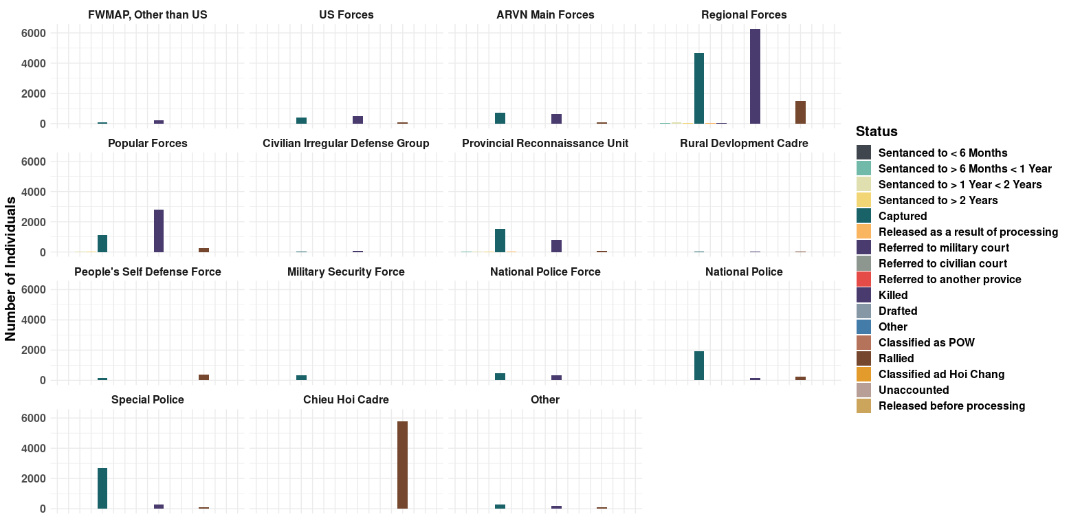
This same data can also be broken down in a few interesting ways. We can plot
the same STATUS data but split into into subplots based on the FORCE that
was responsible for the (coldly bureaucratically termed) neutralization.
 \
\
Using this plot, we can see that “Regional Forces” where the most active group, with “ARVN Main Forces”, “Popular Forces”, “Provincial Reconnaissance Unit” making up much of the remainder.
This plot also shows that US Forces, at least according to this database, where not as nearly as directly involved as organizations that can be grouped into the “South Vietnamese Allies” category.
Lastly, I was interested in what this program looked like over time. Individuals
that were captured (opposed to killed outright) usually had a value in their
SADATX field: “Date of sentence action in YYMM order”. I used this as a proxy
for a given group’s activity over time, granted this would be easily skewed in
the case one group was tasked explicitly with capturing while another was tasked with killing.
Plotting SADATX vs the number of individuals for all groups listed by the FORCES field
produced the plot below.

There is still much to be said
I only looked at a small part of this dataset, but there is still much more to be gleaned. If you would like to play around with the data yourself you can download the csv file I produced from this link. You can also download all the documentation I referenced from the National Archives entry at this link.
Thank you for reading.
-eth